1. Introduction
The most significant difference between retrospective cohort studies and randomized controlled trials (RCTs) compared to cross-sectional studies lies in their temporal characteristics.[1] In cohort studies, not only is a certain phenomenon (Y) important, but the analysis of the time it takes for the phenomenon to occur (time-to-event) is also crucial.[2] However, when analyzing the time-to-event values, it is essential to consider that not all observations are complete data. The term “complete” used in this study refers to securing the same observation period for all patients without censoring.[3] For example, there can be a situation where we designed a study to evaluate the effects of a specific drug on cancer patients’ survival.[4] In this case, equally important as survival or death (Y = 0 or 1) is the survival time (time-to-event until death) for both group T (treatment group) and group C (control group). Thus, the dependent variable is a pair of outcome and survival time.
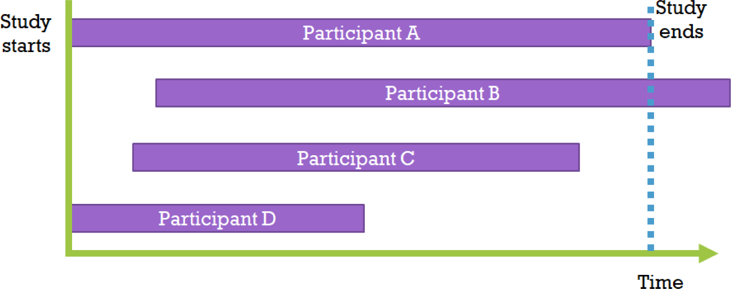
However, when comparing the survival time values of patients in group T and group C using the t-test of the average survival time variable, the following issue arises[5]: “Should we exclude all data in cases where loss to follow-up occurred due to accidents, moving, tracking failure, research fund exhaustion, or death of observers?” Patients’ observation periods can be reduced for various reasons, which is defined as censoring.[6] Since indiscriminately removing censored data can lead to bias issues, statistics that include this censored data must be used. Moreover, as some patients may have different starting points for the study, the initial observation starting point and end point for each patient can be very diverse as shown in the figure (Fig. 1). Survival analysis is a research method that targets both survival time and observation results in order to solve all these problems.[7]
2. Main: survival analysis
Survival analysis tools treat an individual’s survival time T as a random variable. That is, various survival analysis functions are defined and used for arbitrary values (survival time t) that the random variable T can take. These survival analysis functions include the following:
-
Survival function. S(t) = P(T > t) is a function representing the probability of being alive at a specific time point t, which means the probability of event time T being greater than t if the sample has not died on the research start date, S(0) = 1. As t in S(t) increases, the value of S(t) either remains the same or decreases (monotonically decreasing characteristic).
-
Lifetime distribution function. F(t) = 1–S(t), which is the probability that an event has occurred up to a specific time point t, opposite to the survival function. The lifetime distribution function F(t) is a type of cumulative function. The function f(t), which is the original form of this cumulative function, is the derivative of F(t) with respect to time, and is called the survival distribution density. f(t) can be interpreted as the death rate per unit time at the time point t.
-
Hazard function. h(t) = f(t)/S(t). This is the conditional probability that an event will occur immediately after surviving up to time t. The probability of an individual survivor who has survived up to day t and dying on day t is obtained by dividing the number of deaths occurring on day t, f(t), by the number of survivors remaining alive up to day t, S(t). Also, there is a cumulative hazard function H(t), which is the integral function of h(t).
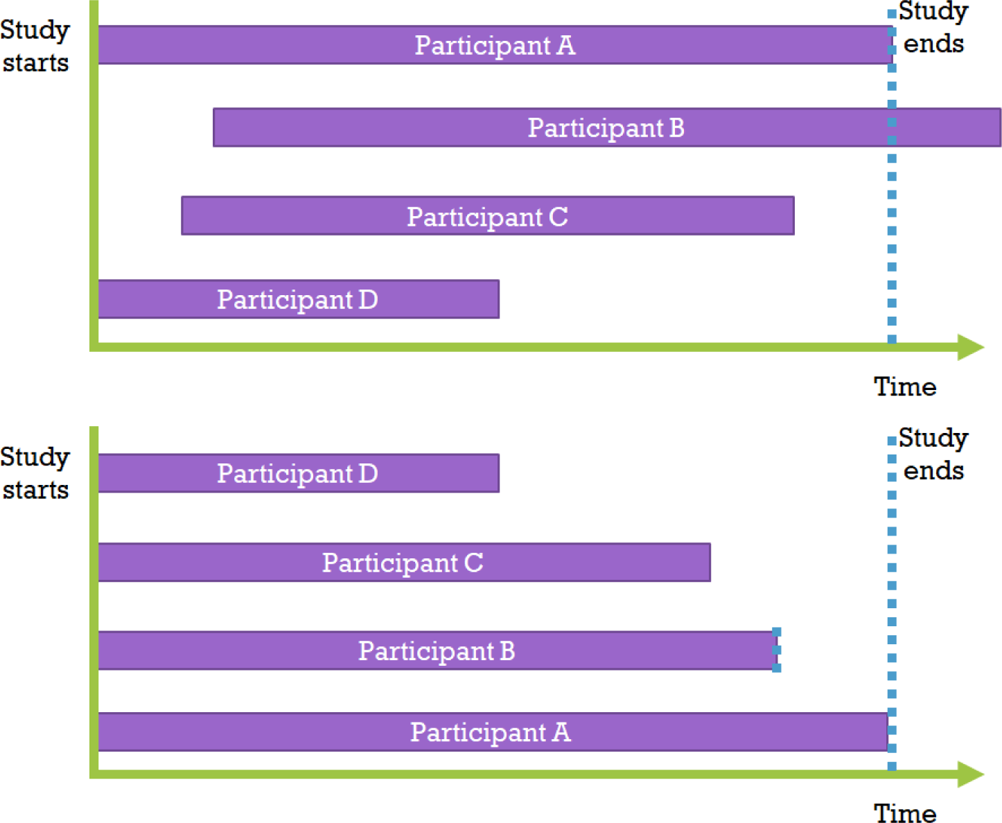
Kaplan-Meier survival analysis is a statistical technique for estimating the survival function. It corresponds to non-parametric statistics, which means that it does not assume parameters and calculates probabilities directly from the given data, regardless of the population’s distribution shape. In other words, it does not include normal distribution assumptions, allowing more general use of the data. According to the Kaplan-Meier estimator method, the data is first arranged in order from the shortest to the longest observation period, and then the starting points are all aligned to 0 (Fig. 2).
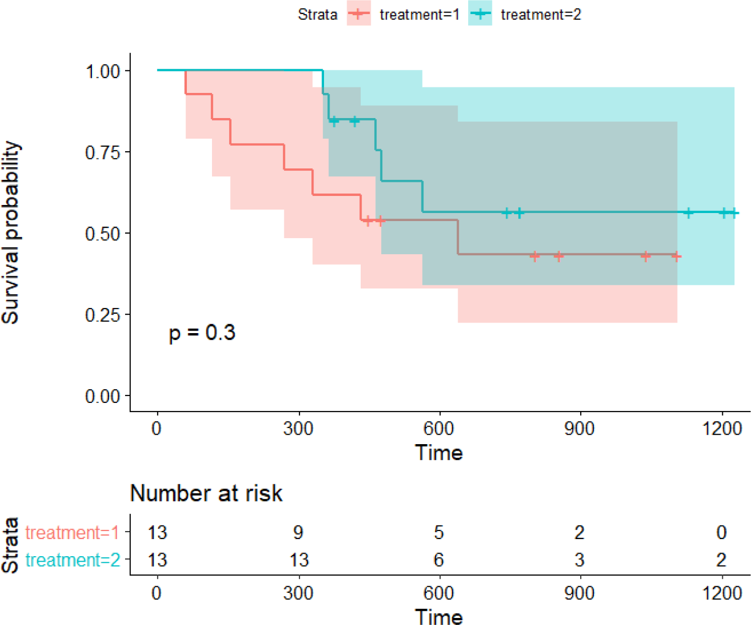
Examining the following example can help understand how to interpret the results of survival analysis in practice. The attached Cancer.csv file is Edmunson’s ovarian cancer research data (Table 1) [8]. Applying Edmunson’s study, we examined whether patients who used a newly developed anticancer drug for ovarian cancer (treatment = 2) survived longer than those who used the existing anticancer drug (treatment = 1) using Kaplan-Meier analysis. The observation time (variable name: time) is the number of days from the start of treatment to the occurrence of death or the end of follow-up.
First, the load of the survival library in R and change of the research outcome pair, survival time and survival status, into a special variable (Surv). Then, the survival results (Surv) can be fitted to the Kaplan-Meier method according to the treatment group. The last line is the code that fit this into the Survfit function, which will obtain the resulting model f1.
In most cases, survival analysis compares the Kaplan-Meier survival curves of two groups. The comparison method used is the log-rank test, with the alternative hypothesis that the survival curves of the treatment and control groups are different. When comparing three or more groups, each are compared using the post-hoc test adjustment. The following is the code to visualize the results of survival analysis using the Survminer library in order to obtain confidence intervals and to obtain the P-value of the log-rank test.[9]
When looking at the results of the code execution in terms of simple survival, it can be found that the new drug treatment group appears to have survived longer. However, the graph shows an overlapping of 95% confidence intervaks, and furthermore, the log-rank test outputs P-value=0.3. In conclusion, it is determined that the new drug did not significantly increase survival (Fig. 3).
The fact that the proportional hazards assumption is a prerequisite for using the log-rank test described above must always be taken into consideration as it is the assumption that the hazard ratio remains constant throughout the study period. A constant hazard ratio means that the mortality rate of the treatment group/control group is always constant from day 1, day 2, ..., until the end of the study.
Kaplan-Meier survival analysis focuses only on the observation period and the occurrence of events. Therefore, other risk factors (such as gender and age) are not considered. Having no covariates in actual medical practice, not experimental studies, is rare. Nonetheless, in an RCT case, variables other than placebo and treatment drugs are randomly assigned and can be excluded from the model, so it is often used in such cases. However, in most studies where the match of other covariates cannot be assured, the Cox proportional hazards regression model, which will be discussed later, should be used.
The basic Cox proportional hazards regression model assumes, like the Kaplan-Meier survival analysis, that the hazard ratio remains constant. The difference from it and the Kaplan-Meier survival analysis is that Cox proportional hazards regression models can analyze other variables that affect the occurrence of events. This is often the reason why the Cox proportional hazards model is used in most data studies.[10-13]
In the proportional hazards regression model, unlike the Kaplan-Meier analysis, an assumption about the original form of the survival function is needed. In the Cox proportional hazards regression model, this function is assumed to be an exponential function, such as s(t)=exp(–kt). Also, the hazard ratio must always be constant over time, which is called the proportional hazards assumption.[14]
Under such assumptions, like in ordinary regression analysis, the hazard ratio of each covariate can be estimated and significant results can be obtained. In most cases, the hazard ratio can be interpreted in a similar way to the relative risk. The significance is evaluated based on whether the confidence interval includes 1 or not, and the value of the hazard ratio itself is given a quantitative meaning.[15]
After analyzing the Cox proportional hazards regression model, survival functions and cumulative hazard functions are graphically represented as in the survival analysis. Similarly, it is common to display censored data, the number of survivors at each time point, etc. It is also often necessary to represent figures most commonly used for testing the proportional hazards assumption, such as the log minus log plot.[16] The log minus log plot is a graph that performs log-log transformation on the survival function and outputs it for each value of the categorical variable; if there is an intersection in the graph, it can be determined that the proportional hazards assumption has been violated.[17]
If an intersection is confirmed in the log minus log plot, the proportional hazards assumption is violated, meaning that the hazard ratio changes over time. In such cases, the time-dependent Cox regression can be performed to analyze changes in variables over time.[18] In fact, many clinical variables strictly correspond to time-dependent variables.[19] Vital sign values, blood test values, etc., are typical examples of time-dependent variables that change over time. Moreover, even if there is a constant value without time-dependency, a time-dependency could be hidden; for example, even if the same drug dosage is set daily, its effect may decrease as resistance develops.[20]
When dealing with time-dependent variables, it may be appropriate to divide them based on the time-dependent cycle and assign them to each observation period. For example, in a study that checks for deaths on a daily basis and performs blood tests every week (every 7 days), data can be split at 7-day intervals and the method of using the blood test value variables for that week is possible.[11, 21]
3. Conclusion
Survival analysis has established itself as a very crucial research methodology in the medical field where observation time is important. Through survival analysis, such as the Kaplan-Meier analysis, the incidence of each group over time can be verified, and testing the differences between groups is possible. Furthermore, by using the Cox proportional hazards regression model, the hazard ratio of each group can be estimated quantitatively. As it is also possible when covariates are present, such methods are very useful for real world data research. However, testing the proportional hazards assumption, such as with the log minus log plot, is necessary in the progress. Finally, time-dependent Cox regression can be used for data with time-dependency using the time-dependent Cox regression.


