1. Introduction
Researchers can conduct an experiment or collect data to study a specific research interest. Meanwhile, it is also possible to perform an analysis that synthesizes the existing research, which is called a meta-analysis. This type of research systematically combines the results of multiple studies on the same topic. This is one of the most prominent features of the characteristics that constitute “a systematic review and meta-analysis.” phrase in the title.
The term “meta-analysis” was first coined in 1976, and the research in this field has grown explosively, especially in the medical field, since the 1990s.[1] Meta-analysis is of particular importance because a myriad of studies has been conducted by different groups in recent years. However, there are some cases in which studies on the same topic have significantly different values and even contradictory outcomes. Therefore, there are inherent limitations when the study only utilizes a single study, as opposed to a meta-analysis.
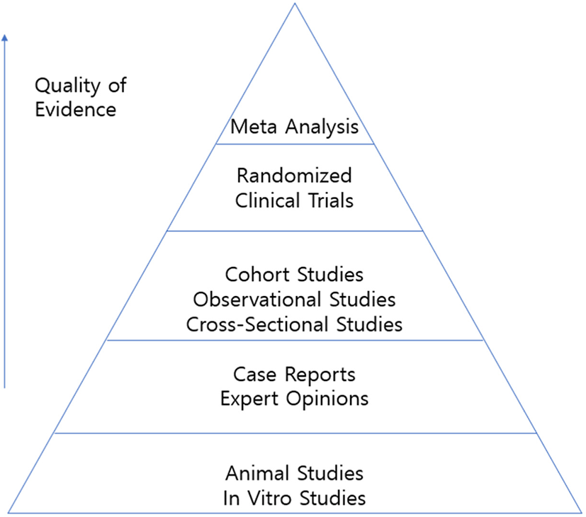
The Cochrane Database of Systematic Reviews was developed in 1994.[2] Since then, most reviews have transformed from the narrative review that relies on subjective opinion into the current systematic review. This trend coincides with modern evidence-based medicine, which emphasizes the accuracy and validity of the data (Fig. 1). The meta-analysis is at the top of the pyramid above case report, retrospective study, prospective study, and randomized clinical trial. Thus, a well-designed meta-analysis has the potential to elicit significant results in medical decision-making.[3]
2. Main: Steps of a meta-analysis
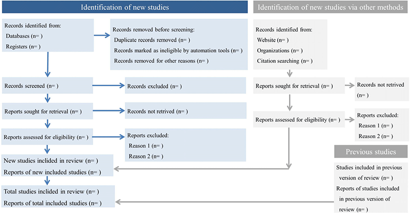
Since meta-analysis integrates several studies, it is essential to choose the appropriate studies. This undergoes a rigorous selection process known as the Preferred Reporting Items for Systematic Reviews and Meta-Analyses (PRISMA).[4, 5] The PRISMA process consists of 1) identification, which identifies the potential database, 2) screening, which removes studies without appropriate intervention methods, duplicated studies, missing comparison groups, and irrelevant studies, 3) eligibility, which reviews full-text and excludes any inappropriate studies, and 4) inclusion, which selects the final studies that will be utilized in the meta-analysis (Fig. 2).
In the identification process, it is recommended that the search strategy is described in detail and then proceed to the initial search. In order to avoid publication bias, public databases, references, and keywords need to be extensively searched. Researchers are also advised to include the grey literature. It is suggested that using publications management programs like Endnote will be convenient to exclude duplicated literature.
The process of reviewing the full text should be performed in accordance with the PICOS framework. This is an abbreviation of the population (or participants), intervention, comparison, outcomes, and study design.[6] Through this, we can also evaluate whether the scope of study subjects, treatment method, control group selection method, outcome variable, and study design satisfy our intention. It is necessary to present included and excluded studies separately to ensure no arbitrariness.
3. Calculating the Effect Size of Each Study
Next, the effect size (ES) of each study should be obtained. The idea of ES is from a classic study by Smith & Glass, and they used the equation below, referred to as Glass’s delta.[7]
The ES gave us a standardized dimensionless effect-representing value that can be obtained regardless of the scale, number of participants, and setup of each study. Since then, multiple methods to obtain ES have been developed. This will be discussed shortly.
The method of obtaining the ES is generally divided into two types depending on whether the outcome (dependent variable) is dichotomous or continuous. The results of dichotomous are displayed in odds ratio (OR), relative risk (RR), or risk difference (RD).[8] However, the continuous results are indicated by the mean difference, standardized mean difference, or correlation coefficient.[9]
First, let us find whether the outcome variable is dichotomous. It is assumed that the experimental results and total numbers of each group are as follows.
Here, the OR value is ad/bc, while RR is an2/cn1. RD is less common, and it means a/n1-c/n2. If researchers understand the above equations, they are able to reverse calculate the remaining values even if only partial values are presented in each row.
When the study outcome is a dichotomous variable, the most used method is performing logistic regression analysis to obtain ORs. Therefore, the standard method to analyze the dichotomous outcome is to convert the results into OR if some are presented in RR or RD. This can be done using the above table and equations (Table 1). Then, we can calculate the ‘log-odds ratio,’ which is the natural logarithm of the OR. This has a mathematical advantage because this converts the ratio into a normally distributed value where zero is the reference. This value (log OR) is the ES. Sometimes, individual research may be unified into RR instead of OR, and in this case, a log RR should be obtained to find ES.
| Event | No event | Total | |
|---|---|---|---|
| Treatment group | a | b | n1 |
| Control group | c | d | n2 |
There are various methods to find the ES when the variable is continuous. The most common way is to find the average and standard deviation of both the treatment and control groups and the p-value difference between them. The ES value is often used in the continuous outcome study by diving the mean difference by the pooled standard deviation instead of the standard deviation of the control group. This is also valid in Glass’ delta as described above. The equation is as follows.
This is called Cohen’s d. The pooled standard deviation can be obtained from the standard deviation of the treatment group (S1) and control group (S2) as follows.
Cohen’s d can also be calculated from t or F statistics, and even p-value. This is because the p-value is a function of degrees of freedom (=n1+n2-2) and t. Thus, the t inverse function gives the t statistics given the p-value and the degrees of freedom. If the p-value is incorrect and/or is expressed vaguely (e.g., P<0.05), request an exact p-value from the original author or use the value next to the inequality sign (e.g., if P<0.05, consider it as p=0.05).[10]
Some studies have suggested the standard error (SE) of SMD and SMD itself instead of the mean and standard deviation, and in this case, it can be thought that Cohen’s d (=SMD) and its variance (square of SE) have already been obtained.[11] However, in order to obtain the average ES, the total number of each treatment group (n1) and control group (n2) must always be secured.[11]
Cohen’s d tends to be overestimated when there are a few samples. There is a way to correct this. A value called Hedge’s g is a calibrated version of Cohen’s d. When the sample size is around 60, the values are almost identical (about 99%), however; when the number is less than 20, the value tends to get smaller. Therefore, Hedge’s g is recommended when the sample size is small. The equation is as follows.
Note that the correction factor inside the parentheses should always be less than one, and the value converges to one as the sample size increases.
Finally, let us find the ES in a study with a correlation coefficient. This is rare among continuous outcome variables. In this case, the ES is simply the correlation coefficient itself. Likewise, most correlation coefficient studies obtain Pearson’s correlation coefficient, often referred to as an r. Instead of using this ES, it can be used as the ES by performing Fisher’s Z transformation. This has a mathematical advantage because the ES gets closer to the normal distribution curve.
4. Calculating the average effect size
When the ES of each study is obtained, the next step is to obtain the average ES. Before starting the calculation, researchers should choose between a fixed effect model and a random effect model.[12] The fixed effect is used when individual studies are conducted in relatively similar conditions. Since the actual ES in each study is similar, the fixed-effect model can be used to estimate the effect value. On the other hand, a random effect model is used when each study is not conducted under the same conditions. Since the actual ES is subject to change, each study is assumed to follow a specific distribution, such as a normal distribution.
Overall, the fixed model is considered more conservative since it has a wider confidence interval for the average ES compared to the random effect model that considers intra- and inter- variations. If the researcher is unsure about the consistency of the ES, using a random effect model is recommended.
The average ES (overall ES) is the weighted average of the ES of all studies. The weight can be determined by several criteria, and the inverse variance model is commonly used. Variance tends to decrease with larger sample sizes. This means that studies with a large sample size tend to have more significance because of the accuracy and validity of the results.
We will see how the variance is calculated in the order of dichotomous outcome, continuous outcome, and correlation coefficient research.
When the researcher uses log OR as an ES, the variance becomes:
When the log RR is used as the ES:
In case of the continuous outcome, the variance of Cohen’s d becomes:
Similarly, the variance of Hedge’s g is:
In the case of correlation coefficient research, if the original Pearson’s correlation coefficient is used as an ES:
If Fisher’s Z is used as an ES:
The weight of each ES can be obtained as the reciprocal of the variance obtained from the above formulas. This is called the inverse variance method. Then, the average ES can be calculated as a weighted average as follows:
Wi and Vi are the weight and variance of the i-th study. M is the final average ES.
In the fixed-effect model, in addition to the inverse variance described above, there are two more options for weights in the dichotomous outcomes. The first one is the Mantel-Haenszel method. This provides a more accurate estimate when the number of samples is small or the event occurrence rate is low. Here, the weights are as follows:
Ni is the total number of participants (i.e., n1+n2) of the i-th study. Then, the average ES is:
However, in this case, M and ORi are not log OR, but the original OR. The second is Peto’s log OR, which can only be used to replace when OR (not RR). This provides more accurate estimates when dealing with rare events less than 1%. Detailed mathematical details will be omitted here.
When using the random effect model, there are no other popular options for calculating average ES except DerSimonian-Laird (DL) method.[13] This paper does not cover detailed methods of DL, but in short, it is a method of estimating tau-squared with Q statistics.
When the average ES is calculated, we also would like to calculate the SE of the average ES. The SE for inverse variance is:
The SE for Mantel-Haenszel is much more complicated and would be omitted here.
Finally, researchers can also calculate the Z-score (not Fisher’s Z but normal distribution) and P-value of the average ES as follows:
5. Forest plot
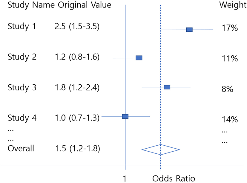
The Forest plot visualizes all studies used in the meta-analysis with the overall ESs in a single figure. Each row shows the ES of each study and the 95% CI of the ES. And in the last row, the average ES obtained from the meta-analysis and the 95% confidence interval of it are displayed.[14]
In order to draw a forest plot, first, the ES of each study and the CI of ES are displayed. This can be obtained by adding 1.96 SE and subtracting 1.96 SE from ES. The weight for each study is also indicated at the end of each row of the forest plot, and in this case, it can be seen that studies with a narrow CI usually have low variance and high weight.
The aggregated ES, which is the average ES obtained by a fixed-effect model or random effect model, will be displayed in the bottom row. Like individual studies, the CI of the average ES will be also indicated by the M - 1.96*SEM and M + 1.96*SEM. In addition, vertical dotted lines can be marked on the average ES value to comfortably see whether the variance of an individual study is larger or smaller than the total ES.
However, some researchers may want to draw forest plots using original values instead of ES. This usually occurs frequently in dichotomous outcome studies. While the log OR is usually obtained as ES, forest plots are expressed as original OR to make it easier for readers to understand (Fig. 3). In these cases, each row of the study represents the OR and CI of the original, and in the last line value will be exp(M), exp(M − 1.96*SEM) and exp(M + 1.96*SEM). The same goes when researchers want to express meta-analysis using log RR as the original RR.
This transformation to the original value also often occurs in the case of correlation coefficient research. If a researcher used Fisher’s Z as an ES, then it can be transformed back to Pearson’s correlation coefficient (r) as follows.
This will give the last line values as r, r − 1.96*SEM and r + 1.96*SEr.
6. Conclusion
Meta-analysis is an interesting research methodology that provides the highest level of evidence. The significance of meta-analysis is that a significant average ES can be obtained even if the study has several limitations. The result also changes with the various methods of obtaining the average ES as explained in this article. Researchers are recommended to thoroughly understand the basic principles of meta-analysis as described in this paper and then perform meta-analysis using related programs and packages.


